
At first glance, Mean Time Between Failures (MTBF) and Mean Time To Failure (MTTF) seem obvious. Hold on, though. Not so fast. To be clear, MTBF/MTTF is a relatively complex metric. Let’s explore this further.
Fundamentals of MTBF and MTTF
Differentiating MTBF vs. MTTF
To start, let’s differentiate MTBF from MTTF. We typically monitor MTBF for repairable items, and we track MTTF for replaceable items. For example, we would employ MTBF to trend the reliability of a centrifugal pump. However, we would employ MTTF to trend the reliability of the pump’s drive-end (DE) bearing.
System, Component, and Part-Level Considerations
This reveals a key complexity of the MTBF/MTTF metric. We must monitor asset reliability at the system, component, and part levels.
In our centrifugal pump example, track the system’s reliability. This includes the pump, motor, coupling, MCC, and both inlet and outlet piping.
In addition, we must monitor the performance of all those components individually, along with various parts associated with each component’s assembly. For defined-level analysis, add the running time, cycles, or miles for both failed and unfailed items. Then, divide that total by the number of failures observed (see figure below).
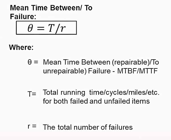
The formula for calculating MTBF and MTTF.
Variability in Failure Metrics
Role of the Arithmetic Mean and Variance
The average, or the arithmetic mean, is the first moment of the probability distribution. It is a measure of central tendency. Median and mode are also measures of central tendency. When one thinks of the mean or average value, the familiar bell-shaped curve of the Gaussian distribution comes to mind.
The distribution is typically bell-shaped when the mean, median, and mode are approximately equal. (NOTE: Although exceptions to that rule exist, they’re beyond this article’s scope). A measure of central tendency, such as MTBF/MTTF, without a measure of variability about that mean can be very misleading and lead to poor decisions.
Averages without measures of variability can be dangerously misleading.
If an asset has a 1,000-hour MTBF/MTTF, one may choose to schedule maintenance before reaching 1,000 hours. For instance, consider 800 hours as a rebuild or replacement time.
Without knowledge of the variance, the second moment of a probability distribution, a reasonable decision can’t be made about that 1,000-hr. MTBF/MTTF.
Standard Deviation and Its Implications
From variance, we derive the standard deviation, which is calculated as the square root of the calculated variance. In our example, the standard deviation around a 1,000-hour MTBF/MTTF is 70 hours. Therefore, an 800-hour rebuild or replacement decision is sound.
Standard deviation turns raw averages into actionable maintenance schedules.
That’s because to be 95% confident about taking action before a failure, we would multiply the standard deviation by 1.65 and subtract that from the MTBF/MTTF. Subtracting 115.5 from 1,000 equals 884.5. Therefore, an 800-hr. rebuild or replace decision would be safe.
On the other hand, what happens if the MTBF/MTTF is 1,000 hours and the standard deviation is 700? In this case, we must subtract 1,155 from 1,000 to determine a suitable rebuild or replace time. But that results in a negative number. Probabilistically, one could not even start the machine in question. This is not reasonable.
Failure Risk Profiles Over Time
In addition to considering the variability of the MTBF/MTTF, we must also consider the failure-risk profile as a function of time (see figure below). Some machines, including components and their parts, experience a higher risk of failure when they’re new.
Such events are sometimes called early-life, infant, or “burn-in” or “run-in” failures. In other instances, we observe a constant risk of failure over time. In other cases, the failure rate will gradually increase or geometrically increase as a function of time.
Understanding the risk profile as a function of time is essential for making informed and effective asset-management decisions. Those different risk profiles as a function of running time/cycles/miles/etc. create very different probability distributions.
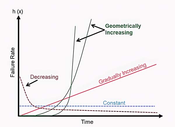
Different failure risk profiles as a function of time.
Applying Weibull Analysis
Reliability engineers employ Weibull analysis to understand the risk profile as a function of time for equipment assets, their components, and the parts for those components.
Understanding the Beta Shape Parameter
The Beta Shape Parameter (β) is an essential output from Weibull analysis.
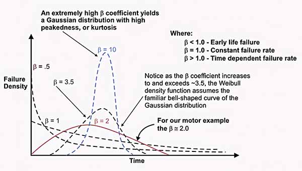
Various probability distributions for different Beta (β) Shape Parameter values.
As the figure above shows, when the β is less than 1.0, the system/component/part experiences early life failures. The closer the β shape parameter is to zero, the stronger the early-life failure risk.
When β is approximately equal to 1.0, the failure rate is constant as a function of time. When β is roughly equal to 2.0, the failure rate linearly increases as a function of time, producing a skewed Rayleigh distribution.
Weibull analysis transforms raw data into clear risk profiles.
Skew is the third moment of the probability distribution. When the β shape parameter equals about 3.5., the distribution assumes the familiar bell shape of the normal or Gaussian distribution.
When the β shape parameter exceeds 3.5, the coefficient of variation decreases, and the bell curve tightens. Consequently, the kurtosis – the fourth moment – increases.
A decision to rebuild or replace an asset, its components, or the parts of those components based on running time/cycles/miles/etc. only makes sense when the β shape parameter is well above 3.5.
Beyond Averages: System Complexity
Despite the apparent elegance of MTBF/MTTF as a metric (largely because of its simplicity and ease of calculation), it may not always support informed and effective asset-management decisions and associated actions.
Previously, I discussed that the failure rate sometimes decreases, sometimes remains constant, and sometimes increases as a function of running time/cycles/distance.
ISO 14224 Framework for Data Collection
Adding to that complexity, most assets and systems of assets are very complex and subject to a wide array of failure modes. The ISO 14224-2016 standard offers an excellent framework for collecting reliability data. Although the standard is written for the petrochemical industries, it is highly applicable and adaptable to any industry.
Collecting data at multiple levels empowers proactive decision-making.
Reliability and asset-performance data should be collected at both use/location and equipment subdivision levels. ISO 14224 suggests collecting use/location data at the industry, business category, installation, plant/unit, and section/system levels. Data collected at this level will likely inform general business-related metrics, not asset reliability.
However, when one drops to the equipment subdivision foundation of ISO 14224, equipment-asset-reliability metrics become paramount. An asset can experience failures at the equipment unit, subunit, component/maintainable item, and/or part level.
Collecting data at all levels is vital for making effective decisions. Still, it’s essential to correctly collect and stratify the equipment/subdivision data levels to drive asset reliability. A wide range of factors could drive MTBF/MTTF for an asset at the equipment unit level.
For example, a sales and marketing team might have committed to a product configuration that exceeds the equipment’s operating capacity, which could lead to a marketing-induced failure.
Or a plant might experience a power outage or disruption of its raw-material supply chain, which could disrupt production (the equipment is failed).
However, the solutions in those cases don’t reside at the equipment-asset reliability level. Thus, including that data in our failure rate and subsequent MTBF/MTTF calculations would have a muddling effect.
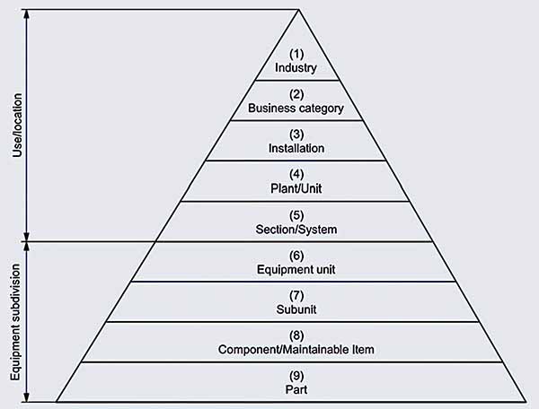
Asset reliability data collection pyramid from ISO 14224:2016.
Granular Analysis in Equipment Subdivisions
Even at the equipment subdivision level of data collection, MTBF/MTTF can be highly variable. Consider the case of a centrifugal pump, which resides at the component/maintainable item (level 8) on the ISO 14224 hierarchy.
A centrifugal pump comprises an impeller, volute, shaft, bearings, inlet pipe/flange, outlet pipe/flange, seal/packing, base, foundation, coupling, etc. It is coupled to and driven by a motor that includes its own various components and motor-control center (MCC).
Moreover, the pump may also include auxiliary systems, such as an external lubrication system. There’s quite a lot going on, even with basic assets in the plant. Component/maintainable items (level 9) on the hierarchy can experience a wide range of failure modes, as can the parts from which they’re constructed.
Take, for example, the volumes of books and articles about the many failure modes of rolling-element bearings.
When they’re all lumped together, the failure modes at the equipment-subdivision level result in a failure rate and associated MTBF/MTTF metric that is so random and variable that it is all but useless in supporting asset management decisions.
Granted, it’s always great to see MTBF/MTTF increase. But suppose you lack clarity about which forcing functions are driving the improvement. In that case, it’s hard to determine if that improvement is a by-product of smart, effectively executed asset-management decisions or just dumb luck.
Impact of Data Aggregation
When failure data is lumped together, it also produces a randomizing effect on the risk profile as a function of time.
Aggregated failure data randomizes risk profiles and obscures insights.
Referring to the figure below, combine failure modes A, B, and C that exhibit an early-life pattern with modes D, E, and F that show a wear-out pattern. This mix causes the system failure rate to flatten into a constant rate after the run-in period.
The entire system appears to have a constant failure rate when, in reality, only failure mode G exhibits the constant failure rate pattern.
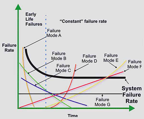
Combining failure data from different components, parts, and failure modes has a “randomizing” effect on the data.
This randomizing effect of combining data at the equipment unit, subunit, component/maintainable item, and part levels in the ISO 14224 standard makes decisions very challenging, especially when different failure modes are at play.
Analyzing Failure Modes Individually
So, taking things one step further, I advise you to collect data and calculate the failure rate and MTBF/MTTF at the failure mode level. Ideally, you’ll collect this data utilizing a standardized taxonomy of failure modes.
The IEC 60812 standard for conducting Failure Modes & Effects Analysis (FMEA) offers an operational-level taxonomy of functional failure modes that can serve as a good starting point (figure below).
The ISO 14224 standard offers taxonomical guidance at a technical failure mode level at the component/maintainable-item level. For mechanical components, I’ve always leaned heavily on the Naval Surface Warfare Center’s (NSWC) Handbook of Reliability Prediction Procedures for Mechanical Equipment. I refer to this 522-page book daily. It can be downloaded for free (see link in the References section below).
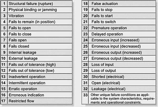
Example taxonomy of functional failure modes from IEC 60812.
Advanced Reliability Analysis
So far, we’ve discussed data collection to support the calculation of failure rates and MTBF/MTTF at the functional, component/maintainable item, and part levels. The concept can be driven down to monitoring the MTBF/MTTF at the root-cause level.
Monitoring our performance at the root-cause level is extremely helpful in driving proactive behaviors in the plant. Monitoring the average time between various root-cause excursions is advanced reliability engineering and asset management.
Apparent Cause Analysis (ACA) vs. Root Cause Analysis (RCA)
Tracking the MTBF/MTTF for root-cause conditions will require your organization to regularly engage in Apparent Cause Analysis (ACA) and Root Cause Analysis (RCA). The first method, ACA, is a simple, scaled-down cause analysis process we employ daily.
Why-Why analysis or Five-Why analysis is a great example of ACA that should be ingrained in your continuous improvement culture. RCA is reserved for more complex and impacting events and near-misses. The difference is that ACA generally employs linear logic by successively asking why there are enough times to arrive at a satisfactory root cause.
With RCA, we start with a universe of all possible causes and systematically eliminate those we know didn’t contribute to the event in question. This approach yields a manageable set of root causes. We know these causes either contributed to the event or cannot be logically eliminated.
Standardized Failure Cause Taxonomies
Whether conducting ACA or RCA, employing a standardized taxonomy of failure cause is helpful. I’ve always found the taxonomy defined in DOE NE 1004:1992 to be very good and generally applicable across industries (see figure below). This is the standard guide for conducting root-cause analysis in the nuclear power industry.
Standardized taxonomies are the backbone of accurate root-cause analysis.
It’s also fully applicable to any RCA investigation. The NSWC book on mechanical reliability serves as an example. This RCA guide was created by the U.S. Department of Energy and is available for free download and unlimited distribution (see References).
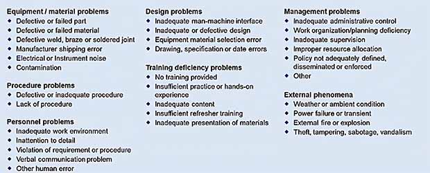
Standard taxonomy of failure causes as defined in DOE NE 1004:1992.
As a lump sum at the use/location level, the usefulness of Mean Time Between/To Failure (MTBF/MTTF) for driving effective asset-management decisions is limited and questionable. As a metric, its usefulness increases at the equipment subdivision level and particularly at the component/maintainable-item-and-part levels.
Plant-equipment systems and processes are complex. Therefore, parse the metric at the failure-mode level to clarify the forcing functions behind MTBF/MTTF improvements or declines.
Effectively compiling data at this level requires sophisticated data-collection hierarchies and taxonomies. Highly sophisticated organizations collect data at the root-cause level to track the average time between excursions in the control of a failure-root-cause condition.
References
ISO 14224:2016. Petroleum, petrochemical, and natural gas industries – Collection and exchange of reliability and maintenance data for equipment. International Organization for Standardization. Geneva, Switzerland.
IEC 60812: 2018. Failure modes and effects analysis (FMEA and FMECA). International Electrotechnical Commission. Geneva, Switzerland.
Naval Surface Warfare Center (2011). Handbook of Reliability Prediction Procedures for Mechanical Equipment. http://everyspec.com/USN/NSWC/download.php?spec=NSWC-11_RELIABILITY_HDBK_MAY2011.055322.pdf
DOE NE 1004:1992. DOE GUIDELINE – ROOT CAUSE ANALYSIS GUIDANCE DOCUMENT. https://www.standards.doe.gov/standards-documents/1000/1004-std-1992/@@images/file