Beyond Weibull: Understanding Recurrence Analysis for Repairable Systems

If you’ve spent time analyzing equipment performance data, you’ve likely encountered the Weibull distribution. It’s a staple in many reliability textbooks and software packages, often the first tool reached for when looking at failure data. Its ability to model various failure behaviors—from infant mortality to wear-out—makes it incredibly versatile, for the right application.

But here’s a critical point that often gets overlooked or misunderstood: the standard Weibull analysis, the kind you use to plot failure data on Weibull paper or fit a distribution to times-to-failure, is fundamentally designed for non-repairable items.

Applying Weibull to repairable systems is like using a single-life lens on a multi-life reality—misleading at best, dangerous at worst.

Applying it blindly to equipment that is repaired and put back into service can lead to misleading conclusions, flawed predictions, and ultimately, poor maintenance and capital expenditure decisions.

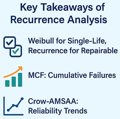
This article explores recurrence analysis, a powerful set of tools specifically designed for repairable systems. We’ll explore why Weibull falls short in these scenarios and how methods like Crow-AMSAA and the Mean Cumulative Function (MCF) provide a more accurate and insightful way to understand the reliability of your most critical assets.

Why Weibull Isn’t Always Your Best Friend (for Repairable Systems)

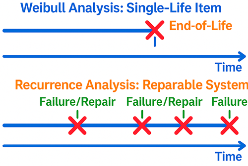
Let’s start by clarifying when Weibull truly shines. For non-repairable items—think components that are discarded and replaced upon failure, like a light bulb, a fuse, or a single-use seal—Weibull analysis is an excellent choice. It allows you to model the time-to-first-failure of these items.

You can determine whether they’re experiencing early life failures (infant mortality), random failures, or wear-out, which helps you make informed decisions about design, warranty periods, and preventive replacement schedules. The underlying assumption is that each item has one life, and its failure signifies the end of its useful existence.

The problem arises when we try to apply this same logic to repairable systems—your pumps, motors, gearboxes, entire production lines, or even a fleet of vehicles. These assets don’t simply fail once and get replaced. They fail, are repaired, and then returned to service, often multiple times over their lifespan.

Consider a pump in a manufacturing facility. It might fail due to a bearing issue, get repaired, and be back online. A few months later, a seal might fail, leading to another repair.

If you simply collect the times between these failures and throw them into a standard Weibull analysis, you’re making a fundamental error. Why? Because each “time-to-failure” after the first isn’t the failure of a new, independent item. It’s a recurring event on the same system, which has likely been impacted by previous repairs, wear, or even improvements.

Using Weibull in such scenarios can lead to several pitfalls:

• Misleading Failure Rate Predictions: You might underestimate the true failure rate of the system over time, as repairs often don’t restore the system to “like-new” condition. Or, conversely, you might mistakenly see an improving trend if repairs are making the system more robust, but Weibull can’t properly capture this.
• Inaccurate Life Cycle Costing: If you misjudge the true recurrence rate of failures, your predictions for future maintenance costs will be off, impacting your budget and capital planning.
• Flawed Maintenance Strategies: Decisions about preventative maintenance, spare parts stocking, and even asset replacement schedules can be suboptimal because they’re based on an incomplete or incorrect understanding of your equipment’s reliability behavior.

Entering the World of Recurrence Analysis

This is where recurrence analysis steps in. Instead of focusing on the time-to-first-failure of an individual component, recurrence analysis is designed to analyze the rate at which events (failures) occur on a system over its operating life. It understands that a system can fail multiple times and that each repair may or may not restore it to its original reliability state.

The beauty of recurrence analysis lies in its ability to handle systems that are continuously put back into service after a repair. It doesn’t treat each failure as the demise of a unique item but rather as another event in the life of a repairable entity.

The two primary tools we’ll explore within recurrence analysis are the Mean Cumulative Function (MCF) and Crow-AMSAA analysis. Both provide unique insights into the reliability of your repairable systems.

The Mean Cumulative Function (MCF): Tracking Cumulative Events

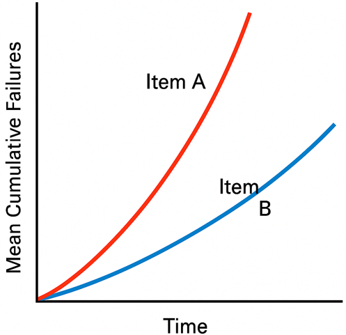
The Mean Cumulative Function (MCF) is a non-parametric plot that shows the average cumulative number of failures (or events) per system over time. It’s an incredibly versatile tool for several reasons:

• No Distribution Assumption: Unlike Weibull, MCF doesn’t assume your failure data fits a particular statistical distribution. This makes it robust and applicable to a wide range of real-world data.
• Comparing Systems/Fleets: You can plot the MCF for different designs, suppliers, maintenance strategies, or even different fleets of assets and visually compare their reliability performance. A steeper slope on the MCF plot indicates a higher rate of recurring failures.
• Predicting Future Failures: By extrapolating the MCF, you can estimate the average number of failures you can expect in the future for a similar system or fleet.
• Assessing Warranty Claims: MCF can be highly effective in analyzing warranty data to determine if a product is failing at a higher rate than expected or if a particular batch has an abnormal failure pattern.

The MCF is calculated by summing the total number of failures for all identical systems up to a certain operating time and then dividing by the number of systems. For example, if you have 10 identical pumps and at 5,000 operating hours, you’ve observed a total of 30 failures across all of them, the MCF at 5,000 hours would be 3.0 (30 failures / 10 pumps).

Crow-AMSAA: Unveiling Reliability Growth or Decay

While MCF tells you the average cumulative failures, Crow-AMSAA analysis (also known as the Power Law Process) takes it a step further by modeling how the rate of failures changes over time.

It’s particularly powerful for situations where you expect reliability to either improve (due to design changes, maintenance improvements, or learning curves) or deteriorate (due to wear, inadequate maintenance, or aging).

Crow-AMSAA is often used in:

• Reliability Growth Testing: During product development, to track if design iterations are successfully improving reliability.
• Field Performance Monitoring: To assess if maintenance strategies are truly reducing failure rates or if aging assets are degrading faster than expected.
• Process Improvement: To see if changes in operational procedures are impacting equipment reliability.

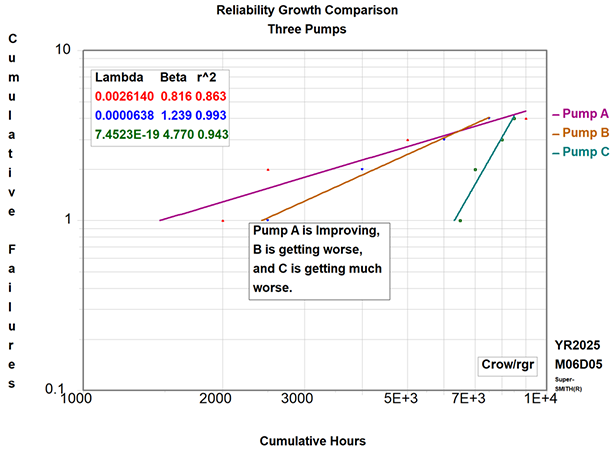
The Crow-AMSAA model describes the intensity function (failure rate) over time using two parameters:

• Lambda (λ): This is a scale parameter that relates to the overall intensity of failures.
• Beta (β): This is the critical shape parameter that tells you about the trend in failure rate:
  • β < 1 (Reliability Growth): The instantaneous failure rate is decreasing over time. This is what you hope to see when you’re implementing effective reliability improvements.
  • β > 1 (Reliability Decay): The instantaneous failure rate is increasing over time. This indicates a deteriorating system or process.
  • β = 1 (Constant Failure Rate): The instantaneous failure rate is constant. This is similar to the “useful life” period of the bathtub curve.

Common Mistakes with Crow-AMSAA:

1. Ignoring the Context: Just getting a β value isn’t enough. You need to understand why it’s greater or less than one. Is β<1 truly due to effective improvements, or is it just the early life of a new system? Is β>1 due to wear or a result of poor maintenance practices?
2. Using it for Individual Components: Remember, Crow-AMSAA is for systems with recurring failures, not for the single-life failure of individual components.
3. Assuming a Constant Rate Prematurely: Don’t assume β=1 without data to support it. Many repairable systems show clear trends.
4. Misinterpreting “Growth”: Reliability growth means the rate of failure is decreasing, not necessarily that there are zero You’re trying to flatten the curve.

Recurrence Analysis in Action: Real-World Examples

Let’s ground these concepts with some practical scenarios.

Example 1: Pump Failures in a Manufacturing Facility

Imagine a manufacturing plant with a critical set of 20 identical centrifugal pumps used in a continuous process. These pumps fail regularly due to various issues (seal leaks, bearing failures, impeller wear) and are repaired in-house. The maintenance team wants to understand if their preventative maintenance program and recent upgrades are actually improving the pumps’ overall reliability.

• Using Crow-AMSAA: The reliability engineer collects all failure and repair times for the entire fleet of 20 pumps, ordered chronologically. A Crow-AMSAA analysis is performed on this pooled data.
  • If the β parameter comes out as less than 1 (e.g., 0.8), it indicates reliability growth. This suggests that the maintenance program, or perhaps specific repair improvements, are successfully reducing the instantaneous failure rate of the pump fleet over time. This insight could justify continued investment in current maintenance strategies or guide further optimizations.
  • If β were greater than 1 (e.g., 1.2), it would signal reliability decay, meaning the pumps are failing more frequently as they age, possibly due to aging infrastructure, inadequate repairs, or increasing operational demands. This would trigger an investigation into potential design issues, the effectiveness of repairs, or the need for capital replacement.
• Using MCF: Separately, the engineer might want to compare the reliability of pumps from two different manufacturers (Supplier A vs. Supplier B) or compare the current fleet’s performance to historical data from five years ago. An MCF plot would show the average cumulative number of failures per pump over its operating life.
  • If the MCF curve for Supplier A is consistently below and less steep than Supplier B, it suggests Supplier A’s pumps are experiencing fewer recurring failures on average, making them a more reliable choice.
  • Comparing the current fleet’s MCF to historical data could visually confirm the effectiveness of the improved maintenance program, showing a flattened, lower MCF curve for the current period.

Example 2: Fleet Management – Delivery Vans

Consider a logistics company managing a large fleet of delivery vans. These vans experience various recurring issues like transmission problems, electrical faults, and brake system failures. The company is interested in evaluating the overall reliability of their fleet, assessing warranty claims for new vans, and optimizing maintenance schedules.

• Using MCF for Warranty Analysis: When a new batch of vans is acquired, the company can track the cumulative failures per van over the warranty period. By plotting the MCF for this batch and comparing it to historical data from previous batches or manufacturer specifications, they can identify if the new vans are underperforming.
  • If the MCF for the new batch shows a significantly higher slope or cumulative failures than expected, it provides strong evidence for warranty claims or a need to re-evaluate the supplier.
• Using Crow-AMSAA for Fleet Maintenance Effectiveness: The maintenance manager wants to know if their investment in advanced diagnostic tools and technician training is paying off by improving the fleet’s overall reliability. They collect all failure events across the entire fleet of vans over a specific period.
  • A Crow-AMSAA analysis on this pooled data could reveal a β value of less than 1, indicating that the average instantaneous failure rate of the fleet is decreasing. This would validate their investment in maintenance improvements and support continued similar strategies.
  • Conversely, if β were significantly greater than 1, it would signal that despite efforts, the fleet’s reliability is degrading, prompting a deeper dive into maintenance efficacy, aging assets, or operational stressors.

Make Smarter Reliability Decisions With Recurrence Analysis

While the Weibull distribution remains an essential tool for analyzing non-repairable items, it’s crucial to recognize its limitations when dealing with repairable systems. For assets that fail, are repaired, and continue to operate, recurrence analysis provides the accurate and insightful framework you need.

Repairable systems live many lives—your reliability analysis should reflect that.

By leveraging tools like the Mean Cumulative Function (MCF), you can effectively compare the performance of different systems, track cumulative failures, and make informed decisions about procurement and warranty claims. And with Crow-AMSAA analysis, you gain the power to model and understand whether your reliability efforts are truly leading to growth, or if your systems are experiencing an undesirable decay in performance.

Embracing recurrence analysis isn’t just about using the right statistical method; it’s about making more informed, data-driven decisions that directly impact your maintenance costs, operational efficiency, and overall asset lifespan. It’s time to move beyond the single-life mindset and truly understand the dynamic reliability of your repairable assets.